3.9. Generating Free Energy Profiles
This tutorial will guide you through the process of generating energy profiles as a collective variable (CV) is modulated with a calculation.
3.9.1. Learning Objectives
Learn how to generate energy profiles with different electronic structure interfaces.
Learn how to generate energy profiles from DataBase queries.
3.9.2. Required Files
The database must be previously generated, and queryable.
The tutorial python script is located in examples/EnergyProfiles
3.9.3. Tutorial
To generate the energy profiles, we will use the calculate_profiles.py script. This is a bit more complex than the previous example, but it is still fairly short.
To start, we will import the necessary modules.
from ase import Atoms
from pymongo import MongoClient
import numpy as np

from rdkit import Chem
from rdkit.Chem import Draw
from pathlib import Path
import matplotlib.pyplot as plt

from pharmaforge.queries import Query
from pharmaforge.interfaces import Scan
from pharmaforge.interfaces import XTBInterface
from pharmaforge.interfaces import Psi4Interface
import time
Now, this script has two modes to be run because it can be a bit slow to run. To start, run the script with
justplot = False
With this option, it will actually run calculations. Note - if it can’t find the xtb or psi4 scans, it will set this back to false and run the calculations so, by default, you can run it with justplot = True and it will run the calculations if they are not found.
3.9.3.1. Ethane-Like Torsional Scan
We will start with a small, ethane-like molecule with a torsional scan.
    try:
        print("Try a torsional scan")
        atoms = Atoms('HHCCHH', [[-1, 1, 0], [-1, -1, 0], [0, 0, 0],
                                [1, 0, 0], [2, 1, 0], [2, -1, 0]])
        newscan = Scan(XTBInterface(method="GFN2-xTB", accuracy=1.0, electronic_temperature=300.0))
        newscan.add_initial_coordinates(atoms)
        newscan.scan(atoms=[1,2,3,4], scan_range=(0,360,20))
        newscan.write_xyz(filename="ethane_scan.xyz")
        print("Scan finished, and an xyz file was written to the current directory as ethane_scan.xyz. You can open it with VMD or PyMOL.")
    except Exception as e:
        print("Calculation failed, skipping test. Is XTB installed? Reason: ", e)
In this code, it generates an ASE Atoms object (with fake coordinates). Then the newscan object calls the XTB Interface and scans the dihedral angle between atoms 1 2 3 4 from 0 degrees to 360 degrees in 20 degree increments. Finally, ethane_scan.xyz is written and can be visualized with VMD.
3.9.3.2. Torsional Scanning with XTB and a Database query
Now, we will try generating a scan from the database query instead. We will start by loading the database, generating a query, and then drawing the molecule with rdkit.
    print("Now lets try it again, but with a molecule from the database")
    try:
        client = MongoClient('mongodb://localhost:27017/')
        db = client["QDPi2_Database"]
    except:
        print("MongoDB is not running, or you haven't created the database in the previous example. Please start MongoDB and try again.")
        exit()


    # This will now grab a molecule from the database, and query it.
    q = Query("nmols eq 1")
    results = q.apply(db, "ani_qdpi")
    mol1 = results[4]
    print(mol1['smiles'])
    print(f"So the molecule we have selected is {mol1['smiles']}")

    # Display the molecule using rdkit
    mol = Chem.MolFromSmiles(mol1['smiles'])
    img=Draw.MolToImage(mol, size=(600, 600), kekulize=True)
    img.show()
![The molecule used for the torsional scan, this is 2-[(thiophen-2-ylmethyltrisulfanyl)methyl]thiophene.](../../_images/torsionalscan_molecule.png)
The molecule is a bit more complex than our first example, but it is still a small(ish) molecule. Its IUPAC name is 2-[(thiophen-2-ylmethyltrisulfanyl)methyl]thiophene, and we will be using it to generate a torsional scan where we rotate one of the dihedral torsions in the chain linking the two thiophene rings.
We will first start by taking one of the first matches from the query and converting it to an ASE atoms object.
    # Convert the molecule to an ASE Atoms object, and grab the first configuration
    atoms = q.result_to_ase(mol1)[0]
    print(f"Created Atoms object: {atoms}")
Now, like before, we will create a newscan object and run the scan, first with XTB. The XTB progrogram is relatively simple to run with the interface built into pharmaforge. In this example, we use the GFN-xTB method.
    print("\n************************")
    print("Now we will perform a torsional scan on the molecule with XTB.")
    try:
        newscan = Scan(XTBInterface(method="GFN2-xTB", accuracy=1.0, electronic_temperature=300.0))
        newscan.add_initial_coordinates(atoms)
        start_time = time.time()
        newscan.scan(atoms=[6, 0, 20, 21], scan_range=(0,360,20), num_workers=1, schedule="bothways", verbose=True)
        end_time = time.time()
        print(f"Scan completed in {end_time - start_time:.2f} seconds.")
        newscan.write_xyz(filename="mol1_scan.xyz")
        newscan.plot_scan()
        # You can access the energies and dihedrals from the scan object.
        xtb_e = newscan.energies
        xtb_dih = newscan.dihedrals
        print("Scan finished, and an xyz file was written to the current directory as mol1_scan.xyz. You can open it with VMD or PyMOL.")
    except Exception as e:
        print("Calculation failed, skipping test. Is XTB installed? Reason: ", e)
When you run the scan, it will show a plot on the screen (if you are normally able to view matplotlib plots). This is the energy profile of the scan.
3.9.3.3. Repeating the scan with Psi4 (Scan Parallelization)
Now, we will do the same thing but with Psi4. The Psi4 interface is similar, but will actually run a DFT calculation. Here we use B3LYP/6-31G, but you can change this to any functional and basis set supported by Psi4. Psi4 supports two methods of parallelization, you can define the number of threads for a single calculation to use with the num_threads argument to Psi4Interface, or you can use the num_workers argument to run multiple calculations in parallel. Timings can be found in the table below.
    print("\n************************")
    print("The same scan, but with psi4 at the B3LYP/6-31G level of theory.")
    try:
        newscan = Scan(Psi4Interface(method="B3LYP", basis="6-31G", num_threads=12))
        newscan.add_initial_coordinates(atoms)
        start_time = time.time()
        newscan.scan(atoms=[6, 0, 20, 21], scan_range=(0,360,20), verbose=True, num_workers=1, schedule="bothways")
        end_time = time.time()
        print(f"Scan completed in {end_time - start_time:.2f} seconds.")
        newscan.write_xyz(filename="mol1_psi4_scan.xyz")
        # The add data option is used to add data from other calculations to the plot.
        newscan.plot_scan()
        psi_e = newscan.energies
        psi_dih = newscan.dihedrals
        print("Scan finished, and an xyz file was written to the current directory as mol1_scan.xyz. You can open it with VMD or PyMOL.")
    except Exception as e:
        print("Calculation failed, skipping test. Is PSi4 installed? Reason: ", e)
Warning
Some interfaces (for instance XTB) utilizes all the vailable threads on the system, so you should not use the num_workers argument with them, by default this will be set to 1. The code has built in checks, and will revert to the serial interface for interfaces that do not support parallelization.
Program |
1 thread, 1 worker (s) |
4 threads, 1 workers (s) |
4 threads, 3 workers (s) |
1 thread, 10 workers (s) |
1 thread, 12 workers (s) |
|---|---|---|---|---|---|
XTB |
18.01 |
N/A |
N/A |
N/A |
N/A |
Psi4 |
1225.97 |
413.84 |
175.09 |
160.91 |
169.02 |
Lastly, we save the data so that we can plot it later without rerunning the calculations.
    xtb_data = np.savetxt("xtb_scan.txt", np.array([xtb_dih, xtb_e]).T, header="Dihedral Energy")
    psi_data = np.savetxt("psi4_scan.txt", np.array([psi_dih, psi_e]).T, header="Dihedral Energy")
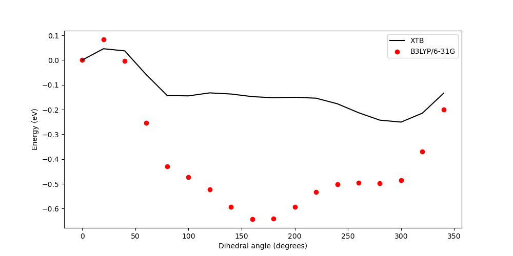
3.9.3.4. Plotting the Final Scan Data
Now, to plot the data set, we can run the same script with the justplot variable set to True.
justplot = True
And the following code will plot the data.
    xtb_dih, xtb_e = np.loadtxt("xtb_scan.txt", skiprows=1, usecols=(0,1), unpack=True)
    psi_dih, psi_e = np.loadtxt("psi4_scan.txt", skiprows=1, usecols=(0,1), unpack=True)

    xtb_e = np.array(xtb_e)-xtb_e[0]
    psi_e = np.array(psi_e)-psi_e[0]

    fig = plt.figure(figsize=(10, 5))
    plt.plot(xtb_dih, xtb_e, label="XTB", c='black')
    plt.scatter(psi_dih, psi_e, label="B3LYP/6-31G", c='red')
    plt.legend(loc="upper right")
    plt.xlabel("Dihedral angle (degrees)")
    plt.ylabel("Energy (eV)")
    plt.show()
This plot, which you should have produced with the above command, looks like this:
3.9.4. Full Code
from ase import Atoms
from pymongo import MongoClient
import numpy as np

from rdkit import Chem
from rdkit.Chem import Draw
from pathlib import Path
import matplotlib.pyplot as plt

from pharmaforge.queries import Query
from pharmaforge.interfaces import Scan
from pharmaforge.interfaces import XTBInterface
from pharmaforge.interfaces import Psi4Interface
import time


justplot = True
if not Path("xtb_scan.txt").exists():
   print("Scan not present, starting from scratch.")
   justplot = False
if not justplot:
    try:
        print("Try a torsional scan")
        atoms = Atoms('HHCCHH', [[-1, 1, 0], [-1, -1, 0], [0, 0, 0],
                                [1, 0, 0], [2, 1, 0], [2, -1, 0]])
        newscan = Scan(XTBInterface(method="GFN2-xTB", accuracy=1.0, electronic_temperature=300.0))
        newscan.add_initial_coordinates(atoms)
        newscan.scan(atoms=[1,2,3,4], scan_range=(0,360,20))
        newscan.write_xyz(filename="ethane_scan.xyz")
        print("Scan finished, and an xyz file was written to the current directory as ethane_scan.xyz. You can open it with VMD or PyMOL.")
    except Exception as e:
        print("Calculation failed, skipping test. Is XTB installed? Reason: ", e)


    print("Now lets try it again, but with a molecule from the database")
    try:
        client = MongoClient('mongodb://localhost:27017/')
        db = client["QDPi2_Database"]
    except:
        print("MongoDB is not running, or you haven't created the database in the previous example. Please start MongoDB and try again.")
        exit()


    # This will now grab a molecule from the database, and query it.
    q = Query("nmols eq 1")
    results = q.apply(db, "ani_qdpi")
    mol1 = results[4]
    print(mol1['smiles'])
    print(f"So the molecule we have selected is {mol1['smiles']}")

    # Display the molecule using rdkit
    mol = Chem.MolFromSmiles(mol1['smiles'])
    img=Draw.MolToImage(mol, size=(600, 600), kekulize=True)
    img.show()

    # Convert the molecule to an ASE Atoms object, and grab the first configuration
    atoms = q.result_to_ase(mol1)[0]
    print(f"Created Atoms object: {atoms}")


    # XTB torsional scan
    print("\n************************")
    print("Now we will perform a torsional scan on the molecule with XTB.")
    try:
        newscan = Scan(XTBInterface(method="GFN2-xTB", accuracy=1.0, electronic_temperature=300.0))
        newscan.add_initial_coordinates(atoms)
        start_time = time.time()
        newscan.scan(atoms=[6, 0, 20, 21], scan_range=(0,360,20), num_workers=1, schedule="bothways", verbose=True)
        end_time = time.time()
        print(f"Scan completed in {end_time - start_time:.2f} seconds.")
        newscan.write_xyz(filename="mol1_scan.xyz")
        newscan.plot_scan()
        # You can access the energies and dihedrals from the scan object.
        xtb_e = newscan.energies
        xtb_dih = newscan.dihedrals
        print("Scan finished, and an xyz file was written to the current directory as mol1_scan.xyz. You can open it with VMD or PyMOL.")
    except Exception as e:
        print("Calculation failed, skipping test. Is XTB installed? Reason: ", e)
    # End XTB scan

    # Psi4 torsional scan
    print("\n************************")
    print("The same scan, but with psi4 at the B3LYP/6-31G level of theory.")
    try:
        newscan = Scan(Psi4Interface(method="B3LYP", basis="6-31G", num_threads=12))
        newscan.add_initial_coordinates(atoms)
        start_time = time.time()
        newscan.scan(atoms=[6, 0, 20, 21], scan_range=(0,360,20), verbose=True, num_workers=1, schedule="bothways")
        end_time = time.time()
        print(f"Scan completed in {end_time - start_time:.2f} seconds.")
        newscan.write_xyz(filename="mol1_psi4_scan.xyz")
        # The add data option is used to add data from other calculations to the plot.
        newscan.plot_scan()
        psi_e = newscan.energies
        psi_dih = newscan.dihedrals
        print("Scan finished, and an xyz file was written to the current directory as mol1_scan.xyz. You can open it with VMD or PyMOL.")
    except Exception as e:
        print("Calculation failed, skipping test. Is PSi4 installed? Reason: ", e)
    # End Psi4 scan

    xtb_data = np.savetxt("xtb_scan.txt", np.array([xtb_dih, xtb_e]).T, header="Dihedral Energy")
    psi_data = np.savetxt("psi4_scan.txt", np.array([psi_dih, psi_e]).T, header="Dihedral Energy")
else:
    xtb_dih, xtb_e = np.loadtxt("xtb_scan.txt", skiprows=1, usecols=(0,1), unpack=True)
    psi_dih, psi_e = np.loadtxt("psi4_scan.txt", skiprows=1, usecols=(0,1), unpack=True)

    xtb_e = np.array(xtb_e)-xtb_e[0]
    psi_e = np.array(psi_e)-psi_e[0]

    fig = plt.figure(figsize=(10, 5))
    plt.plot(xtb_dih, xtb_e, label="XTB", c='black')
    plt.scatter(psi_dih, psi_e, label="B3LYP/6-31G", c='red')
    plt.legend(loc="upper right")
    plt.xlabel("Dihedral angle (degrees)")
    plt.ylabel("Energy (eV)")
    plt.show()